
Article before I knew we had to write about the group project :).
The basics for algorithms
The simple truth is that algorithms are just ways to do things. They’re processes to solve a type of problem. These problems can be complex however, just because there are difficult algorithms doesn’t mean that all algorithms are that complex.
You can begin thinking algorithmically by breaking the problem down and building the solution up, or by breaking the problem down and building the solution up. As developers, we have a natural urge to start with the solution. However, I would recommend breaking down the problem first and then creating the solution from there.
Thinking in small steps to solve a problem takes time. But it will however help us better understand the problem. The better an algorithm is, the shorter the time is to determine that an algorithm is faster, scientists have developed the big o notation later on we go into further detail.
So, how do you even begin to think about these problems to solve in the first place. To solve a problem you always need data. This data we call a dataset this data gives us the possibility to do an analysis. Can I solve my problem with the data as it is now or should I first prepare this data so that it meets my needs. If you have answers to these questions we can start solving our problem. To begin with, it is useful to grab a small sample of your original dataset. With this sample we are going to work out our algorithm
Using that principle for our algorithm, if we can get it to operate correctly with one item entry and then with ten, we can probably get it to work with any number of items. You'll eventually test it with a lot more to confirm. This gradual build-up aids you in comprehending the nuances and identifying the problem's subtle traps. During this process you really get to know the data.
The running time of an algorithm can very with...
- The size of the input
- The content structure of the input
- The type of computer we're using
- The amount of memory the computer has
- How the algorithm is implemented
- The programming language used
Data structures
A data storage format. It is the collection of values and the format they are stored in, the relationships between the values in the collections as well as the operations applied on the data stored in the structure. These stored data collections are called arrays. These arrays can very per language examples of this are The language Java with homogeneous containers type are type bound. In python we have heterogeneous structures they are not type bound.
It often occurs that during an algorithm it is necessary to sort or search for data. For these functions several already existing algorithms / data structures have been developed. Some very well-known algorithms are:
Searching:
- Linear search
- Binary search
Sorting:
- Insertion sort
- Selection sort
- Bubble sort
- Heapsort
- Merge sort
- Quick sort
- Radix Sort
Data structures elements:
- Array n dimensional & Strings
- Boolean
- Trees
- Tuple & Sets
- Hashmap and hashtable
- Linked List
- Stack and Queues
Thankfully, you’ll probably never have to actually implement any of these algorithms as a professional developer. These days, the most efficient search and sort algorithms are provided in standard libraries that come with most languages. But still it is important for you to know how to use one and what the advantages and disadvantages are.
What makes a good algorithm
Correctness
Sometimes a algothim does not give you a correct answer or the best answer because the only perfect algorithms that we know for those problems take a really, really long time. Fore example lets say we want a programm that would determine the most effiecient oute for a truck that delivers packages. staring and ending the day at a depot. It would take weeks to run to going through all the possibilites. But if we're okay with a program that would determine a route that goed but maybe not the best. Then i could run in seconds in some cases, good is good enough.
Efficiency
Asymptotic analysis allows algorithms to be compared independently of a particular pogramming laungauage or handware.
Asymptotic notation
Let's think about the running time of an algorithm more carefully. We use a combination of two ideas. First, we determine how long the algorithm takes, in terms of the size of its input. So we think about the running time of the algorithm as a function of the size of its input. The second idea is that we focus on how fast this function grows with the input size. We call that the rate of growth of the running time. To keep things manageable, we simplify the function to distill the most important part and cast aside the less important parts.
We'll see three forms of it: big-Θ notation, big-O notation, and big-Ω notation.
Big-Θ notation
When we use big-Θ notation, we're saying that we have an asymptotically tight bound on the running time. "Asymptotically" because it matters for only large values of n. "Tight bound" because we've nailed the running time to within a constant factor above and below.
Big O notation
Big-O notation is used by programmers to compare and measure the performance of algorithms. Big O notation is one of the most fundamental tools for computer scientists to analyze the cost of an algorithm. It is a good practice for software engineers to understand in-depth as well. The big O notation gives a strong statement about the worst-case running time. We use big-Θ notation to asymptotically bound the growth of a running time to within constant factors above and below. Sometimes we want to bound from only above. Because big-O notation gives only an asymptotic upper bound, and not an asymptotically tight bound, we can make statements that at first blush seem incorrect, but are technically correct.
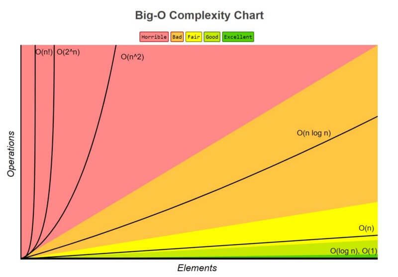
O(1) has the least complexity
If you can build an algorithm that solves the problem in O(1) notation, you are likely at your best possible solution. When the complexity of a scenario exceeds O(1), we can examine it by looking for its O(1/g(n)) equivalent. For instance, O(1/n) is more difficult than O(1/n2).
O(log(n)) is more complex than O(1), but less complex than polynomials
Because sorting algorithms are frequently associated with divide and conquer algorithms, O(log(n)) is a desirable complexity to aim for. Because the square root function can be regarded a polynomial with an exponent of 0.5, O(log(n)) is less difficult than O(n).
O(nˣ) Complexity of polynomials increases as the exponent increases
For example, O(n⁵) is more complex than O(n⁴). Due to the simplicity of it.
O(2ⁿ) Exponentials have greater complexity than polynomials as long as the coefficients are positive multiples of n
O(2ⁿ) is more complex than O(n⁹⁹), but O(2ⁿ) is actually less complex than O(1). We generally take 2 as base for exponentials and logarithms because things tends to be binary in Computer Science, but exponents can be changed by changing the coefficients. If not specified, the base for logarithms is assumed to be 2.
you can write a book about big o notation so much and so big is the subject but for more information I would just google the topic.
Big-Ω (Big-Omega) notation
We might wish to declare that an algorithm takes at least a specific amount of time without specifying a maximum time. The Greek letter "omega" is used in big-Ω notation. We use big-Ω notation for asymptotic lower bounds, since it bounds the growth of the running time from below for large enough input sizes.
Lets begin
Basics
Arrays:
Python = list = non type bound
Java = array = type bound
Executions
Operations on Data structures
- Access and read values
- Search for an arbitrary values
- Insert values at any point into the structure
- Delete values in the structure
We access the data in the array by using the index of the stored positions of the value. Every value in the array has its index with which you can locate it also called an address. The base index in most languages is 0 to n; space = n * m.
new_list = [1, 2, 3]
result = new_list[0]    # 1
result = new_list[10]   # IndexError: list index out of range
You cannot access an address index that is larger than your instantiated array size. This will always result in an index out of bound error.
Lets now search for a value in our list with Linear search:
if 1 in new_list : print(True)

for n in new_list:
    if n == 1:
        print(True)
        break
Lets insert a new value in the array: there are two methods to do so one on linear runtime and on constant time Append. They're different in that insert linear will insert in every given index and append will add to the array. But it also depends on the language we use.
numbers = [] # Default 1 element can be inserted
len(numbers) # Will give 0 as answer
numbers.append(2)
numbers.append(200) # Will execute resize array
The append function will only increase the when the index will hit size 0, 4, 8, 16, 25, 35, 46... and so on we call this amortized constant space complexity.
# Big-O of K | K = Number of items we append
numbers = []
numbers.extend([4, 5, 6]) # Makes a serie of append calls
Linked list
Each data structure solves a particular problem. Arrays are particularly good at accessing/reading values that will happen in constant time. But arrays are pretty bad at inserting and deleting which both run at linear time. Linked lists on the other hand are somewhat better at this although it has some problems. They are trying to solve a problem that involves far more inserts and deletes than accessing. A linked list can be a better tool than an array.
A linked list is a linear data structure where each element in the list is contained in a separate object called a node. A node models two pieces of information an individual item of the data we want to store and a reference to the next node in the list. The first node in the linked list is called the head of the list. While the last node is called the tail. The head and the tail nodes are special the list only maintains a reference to the head although in some implementations it keeps a reference to the tail as well. Every node other than the tail point to the next node in the list. But the tail doesn't point to anything this is how we know it's the end of the list. Nodes are what called self-referential objects. Linked lists usually come in two forms a singly linked list where each node stores a reference to the next node in the list or a doubly linked list where each node stores a reference to both the node before and after
class Node:
    # An object for storing a single node of a linked list
    # Models tow attributes - data and the link to the next node in the         list

    data = None # To hold on to the data we are storing
    next_node = None # To point to the next node in the list

    def __init__(self, data):
        self.data = data

    def __repr__(self):
        return "<Node data: %s>" % self.data # ToString value

class LinkedList:
    # Singly linked list

    def __init__(self):
        self.head = None

    def is_empy(self):
        return self.head == None

    def size(self):
        # Return the number of nodes in the list
        # Takes 0(n) / linear time

        current = self.head
        count = 0

        while current:
            count += 1
            current = current.next_node

        return count

    def add(self, data):
        # Adds new Node container data at head of the list
        # Takes 0(1) time

        new_node = Node(data)
        new_node.next_node = self.head
        self.head = new_node

    def search(self, key):
        # Search for the first node containing data that maches the key
        # Return the node or 'None' if not found
        # Takes 0(n) time

        current = self.head

        while current:
            if current.data == key:
                return current
            else:
                current = current.next_node

        return None

    def insert(self, data, index):
        # Inserts a new Node containing data at index position
        # Insertion takes 0(1) time but infing the node at the insertion point take 0(n time)
        # Takes overal 0(n) time

        if index == 0 :
            self.add(data)

        if index > 0:
            new = Node(data)

            position = index
            current = self.head

            while position > 1:
                current = node.next_node
                position -= 1

            prev_node = current
            next_node = current.next_node

            prev_node.next_node = new
            new.next_node = next_node

    def remove(self, key):
        # Removes Node containing data that matches the key
        # Return the node of None if key doesn't exists
        # Takes 0(n) time

        current = self.head
        previous = None;
        found = False

        while current and not found:
            if current.data == key and current == self.head:
                found = True
                self.head = current.next_node
            elif current.data == key:
                found = True
                previous.next_node = current.next_node
            else:
                previous = current
                current = current.next_node

        return current

    def node_at_index(self, index):
        if index == 0:
            return self.head
        else:
            current = self.head
            position = 0

        while position < index:
            current = current.next_node
            possition += 1

        return current

    def __repr__(self):
        # Return a string representation of the list
        # Takes 0(n) time

        nodes = []
        current = self.head

        while current:
            if current is self.head:
                nodes.append("[Head: %s]" % current.data)
            elif current.next_node is None:
                nodes.append("[Tail: %s]" % current.data)
            else:
                nodes.append("[%s]" % current.data)

            current = current.next_node
        return '-> '.join(nodes)


# [Head],[],[],[],[Tail]
l = LinkedList()
l.add(1)
l.size() # returns 1
l.add(2)
l.add(3)
l.size() # returns 3

l # returns [Head: 3]-> [2]-> [Tail: 1]
Head can be seen as the top of an book pile its the first book you pick from the pile. Unlike arrays where when you insert an element into the array all element after the particular index need to be shifted. With a linked list we just need to change the references to next on a few nodes. This way we can insert a node at any point in the list in constant time.
Merge sort
Merge sort works like binary sort by splitting up the problem into sub problems. But it takes it one step further. In the first sequence we split the array into two smaller arrays on the second sequence we are going to split the first sequence again and so on until we are down to single element arrays. After that the merge sort algorithm works backwards. By repeatedly merging the single element arrays and sorting them at the same time.
Solving a problem like this by recursively breaking down the problem into subparts until it is easily solvable is an algorithmic strategy called divide and conquer.
def merge_sort(list):
    # Sorts a list in ascending order
    # Return a new sorted list

    # Devide: Find the midpoint of the list and divide into sublists
    # Conquer: Recursively sort the sublist created in previous step
    # Combine: Merge the sorted sublists created in previous step

    # Takes O(kn log n) time

    if len(list) <= 1:
        return list

    left_half, right_half = split(list)

    left = merge_sort(left_half)
    right = merge_sort(right_half)

    return merge(left, right)

def split(list):
    # Divide the unsorted list at midpoint into sublists
    # Returns two sublists - left and right

    # Takes overal O(k log n) time

    min = len(list)//2
    left = list[:mid] # list[0:mid]            Takes n of k
    right = list[mid:] # list[mid:len(list)]

    return left, right

def merge(left, right):
    # Merges two lists (arrays), sorting them in the process
    # Return a new merged list

    # Runs in overal O(n) time

    l = []
    i = 0
    j = 0

    while i < len(left) and j < len(right):
        if left[i] < right[j]:
            l.append(left[i])
            i += 1
        elif left[i] >= right[j]:
            l.append(right[j])
            j += 1

    while i < len(left):
        l.append(left[i])
        i += 1

    while j < len(right):
        l.append(right[j])
        j += 1

    return l

def verify_sorted(list):
    n = len(list)

    # Stopping condition
    if n == 0 or n == 1:
        return true

    return list[0] < list[1] and verify_sorted(list[1:])
    # [1, 2, 3, 4, 5]
    # [2, 3, 4, 5]
    # [3, 4, 5]
    # [4, 5]
    # [5]


alist = [54, 62, 93, 17, 77, 31, 44, 55, 20]
l = merge_sort(alist)
print(l) # Return [17, 20, 31, 44, 54, 62, 77, 93]
print(verify_sorted(alist)) # Return False
print(verify_sorted(l)) # Return True
Linked list merge sort
from linked_list import LinkedList

def merge_sort(linked_list):
    # Sorts a linked list in ascending order
    # - Recursively divide the linked list into sublists containing a single node
    # - Repeatedly merge the sublists to produce sorted sublists until on remains
    # Returns a sorted linked list

    if linked_list.size() == 1:
        return linked_list
    elif linked_list.head is None:
        return linked_list

    left_half, right_half = split(linked_list)
    left = merge_sort(left_half)
    right = merge_sort(right_half)

    return merge(left, right)

def split(linked_list):
    # Divide the unsorted list at midpoint into sub linked lists

    if linked_list == None or linked_list == None:
        left_half = linked_list
        right_half == None

        return left_half, right_half

    else:
        size = linked_list.size()
        mid = size//2

        mid_node = linked_list.node_at_index(mid - 1)

        left_half = linked_list
        right_half = LinkedList()
        right_half.head = mid_node.next_node
        mid_node.next_node = None

        return left_half, right_half

def merge(left, right):
    # Merges two linked lists, sorting by data in the nodes
    # Return a new, merged list

    # Create a new linked list that contains nodes from
    # Merging left and right
    merged = LinkedList()

    # Add a fake head that is discarded later
    merged.add(0)

    # Set current to the head of the linked list
    current = merged.head

    # Obtain head nodes for left and right linked lists
    left_head = left.head
    right_head = right.head

    # Iterate over left and right unril we reach the tail node of either
    while left_head or right_head
        # If the head node of left is None, we are past the tail
        # Add the node from right to merged linked list

        if left_head is None:
            current.next_node = right_head
            # Call next on right to set loop condition to False
            right_head = right_head.next_node

        # If the head node of tight is None, we are past the tail
        # Add the tail node from left to merged linked list
        elif right_head is None
            current.next_node = left_head
            # Call next on left to set loop condition to False
            left_head = left_head.next_node

        else:
            # Not at either tail node
            # Obtain node data to perform comparison operations
            left_data = left_head.data
            right_data = right_head.data
            # If data on left is less than right, set current to left node
            if left_data < right_data:
                current.next_node = left_head
                # Move left head to next node
                left_head = left_head.next_node
            # If data on left is greater than right, set current to right node
            else:
                current.next_node = right_head
                # Move right head to next node
                right_head = right_head.next_node

        # Move current to next node
        current = current.next_node

    # Discard fake head and set first merged node as head
    head = merged.head.next_node
    merged.head = head

    return merged

l = LinkedList()
l.add(10)
l.add(2)
l.add(44)
l.add(15)
l.add(200)

print(l)
sorted_linked_list = merged_sort(l)
print(sorted_linked_list)
#[Head: 200]-> [15]-> [44]-> [2]-> [Tail: 10]
#[Head: 2]-> [10]-> [15]-> [44]-> [Tail: 200]

# split -> size
# midpoint = 2
#[Head: 200]-> [15]-----> [44]-> [2]-> [Tail: 10]
#Left : [Head: 200]-> [15]
#SubLeft : [Head: 200]
#SubRight : [Head: 15]
#Current: [Head: 15]-> [200]


#Right: [Head: 44]-> [2]-> [Tail: 10]
These are the data structures I began with, these are the fundamentals for algorithmic.
Recursion
The ability of a function to call itself. Recursive functions are difficult to understand. The flow of control is quite complex.
# Normal
def sum(numbers):
    total = 0
    for number in numbers:
        total += number
    return total

print(sum([1, 2, 7, 9]))
# Recursion
def sum(numbers):
    if not numbers:
        return 0
    print("Calling sum(%s)" % numbers[1:])
    remaining_sum = sum(numbers[1:])
    print("Call to sum(%s) returning %d + %d" % (numbers, numbers[0], remaining_sum))
    return numbers[0] + remaining_sum

print(sum([1, 2, 7, 9]))
# Calling sum([2, 7, 9])
# Calling sum([7, 9])
# Calling sum([9])
# Calling sum([])
# Call sum([9]) returning 9 + 0
# Call sum([7, 9]) returning 7 + 9
# Call sum([2, 7, 9]) returning 2 + 16
# Call sum([1, 2, 7, 9]) returning 1 + 18
# Result: 19
Quick Sort
QuickSort is a Divide and Conquer algorithm. It picks an element as pivot and partitions the given array around the picked pivot. There are many different versions of quickSort that pick pivot in different ways.
List: [4, 6, 3, 2, 9, 7, 3, 5]
Pivot: [4]
Less than pivot: [3, 2, 3] -> [2, 3] [3] [ ] -> [ ] [2] [3] = [2, 3] -> [2, 3] [3] [ ] -> [2, 3, 3]
Greater than pivot: [6, 9, 7, 5] -> [5] [6] [9, 7] -> [5, 6, 7, 9]
[2, 3, 3, 4, 5, 6, 7, 9]
import sys
from load import load_numbers

numbers = load_numbers(sys.argv[1])

def quicksort(values):
    if len(values) <= 1:
        return values
    less_than_pivot = []
    greater_than_pivot = []
    pivot = value[0]

    for value in values[1:]:
        if value <= pivot:
            less_than_pivot.append(value)
        else :
            greater_than_pivot.append(value)

    print("%15s %1s %-15s" % (less_than_pivot, pivot, greater_than_pivot))
    return quicksort(less_than_pivot) + [pivot] + quicksort(greater_than_pivot)

print(numbers)
# [4, 6, 3, 2, 9, 7, 3, 5]
sorted_number = quicksort(numbers)
# [3, 2, 3] 4 [6, 9, 7, 5]
#    [2, 3] 3 []
#        [] 2 [3]
#       [5] 6 [9, 7]
#       [7] 9 []
print(sorted_numbers)
# [2, 3, 3, 4, 5, 6, 7, 9]
Selection sort
Also a bad sorting sorting algorithm. With each loop we will look through each of the values in the unsorted array and find the smallest value and move that value to the end of the sorted array. We start with the first value in the unsorted and say its the minimum or smallest value we have seen so far for now. Than we will look at the next value and see if that one is smaller than the current smallest value if so we mark is as the new minimum. We continue that way until we reach the end of the list. We know that the value that we have marked is the smallest value in the array. Than we move that value from the current list to a new list called sorted and we delete it from the current list. We do this until there are no more items in the unsorted array.
import sys
from load import load_numbers

numbers = load_numbers(sys.argv[1])

def selection_sort(values):
    sorted_list = []
    print("%-25s %-25s" % (values, sorted_list))
    for i in range(0, len(values)):
        index_to_move = index_of_min(values)
        sorted_list.append(values.pop(index_to_move))
        print("%-25s %-25s" % (values, sorted_list))
    return sorted_list

def index_of_min(values):
    min_index = 0
    for i in range(1, len(values)):
        if values[i] < values[min_index]:
            min_index = i
    return min_index

print(selection_sort(numbers))
Bogo Sort
Bad sorting randomly switching numbers till its sorted. Stumbling on a solution is literally a matter of luck and for lists with more than a few items it might never happen.
import random
import sys
from load import load_number

number = load_numbers(sys.argv[1])

def is_sorted(values):
    for index in range(len(values) - 1)
        if values[index] > values[index + 1]:
            return False
    return True

def bogo_sort(values):
    attempts = 0
    while not is_sorted(values):
        print(attempts)
        random.shuffle(values)
        attempts += 1
    return values

print(bogo_sort(numbers))
Thank you for reading this topic about Algorithmics I hope it was interesting any feedback is always welcome. Hope to see you in the next topic,
Byee! 👋🍺
TL;DR What are algorithmics